Kayıtlar

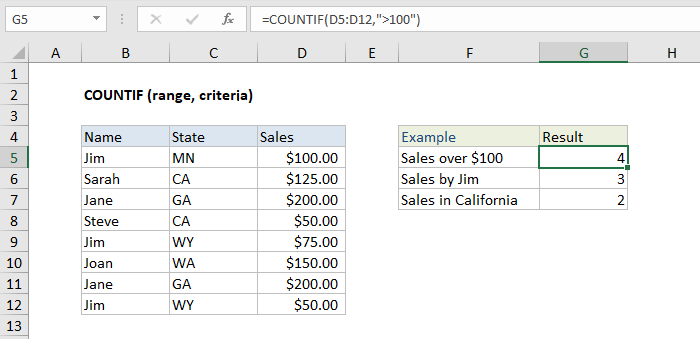
Sum - SUMIF - SUMIFS

Resim
Sum Functions in Excel =SUM(A2:A10) => Adds the values in cells  between A2 and A10. =SUM(A2:A10; C2:C10) Adds the values in cells  between A2 and A10 +  C2 and C10 SUMIF function For example, suppose that in a column that contains numbers, you want to sum only the values that are larger than 5. You can use the following formula:  =SUMIF(B2:B25;">5") SUMIFS  function SUMIFS(sum range; criteria_range1; criteria1; [criteria_range2; criteria2]; ...) =SUMIFS(A2:A9;B2:B9;"=A*";C2:C9;"Tom")

COUNTIF Function in Excel

Resim
COUNTIF "COUNTIF" can be used to count cells that contain dates, numbers, and text. =COUNTIF(D5:D12;">100")  => count cells where greater than 100 between D5 and D12. =COUNTIF(B5:B12;"jim") => count cells where equal to "Jim" between D5 and D12.  =COUNTIF(A1:A10;"<"&B1) => count cells less than B1 & => after quote if you want to write excel variable, type it before the variable. =COUNTIF(A1:A10;"<>red") => count cells where not equal to "red" between A1 and A10.  =COUNTIF(A1:A10;"<"&DATE(2020;4;1)) => count cells where greater than the date between A1 and A10. =COUNTIF(A1:A5;"???") => count cells where contain 3 characters.

Create table in excel

Resim
Create Table 1-Select your data 2-Click "Insert" on menu. 3-Click "Table"  on Ribbon Menu. 4-Click "OK". You can add new column by right clicking the mouse on the column header.Then Click "Insert". +The advantage of the table is that the formula written for any row is added to all rows automatically.And chart creation is easier in the table.If you press "F11" after selecting the table, the chart will open in a new tab. You can add or remove filters on Ribbon Menu by clicking "Sort & Filter". Create Pivot Table 1-Select your data 2-Click "Insert" on menu. 3-Click "Pivot Table" on Ribbon Menu. 4-Click "OK". 5-In the right drop-down menu, you can drag your columns as rows and values.Optionally you can add more rows and values.

What You Need to Know About VLookup Function in Excel

Resim
  VLookUP (Usually used for unique data) 1-First, you choose the cell where you want to add listmenu.Then click "View" on Menu. 2-Click "Data Validation" in Ribbon Menu. 3-Select "List" in Allow Menu. 4-Click "Source" input and select your data where u want to search. Now let's get data according to the variable in the menu. 1-Write " =VLOOKUP( " in function area; 2-Select the list and type ";". 3-Then select all data where we search martial status for matched name with the list. (Name-Martial Status Table) 4-Type ";" again and write the column number we get data from selected table (2.column) 3-Type ";" again and write "0" for exact match.(OR "1" for approximate match)  4-Close the bracket.Then Click Enter. Other method => You can write same function by clicking Fx and fill the form. final formula  : =VLOOKUP(A8;A2:B6;2;0)

Detecting Unique Data in Excel

Resim
Unique Data Filter 1-Click "Data" Tab on Menu.  2-Click "Advanced" next to the "Filter" on Ribbon Menu. 3-Tick "Copy to another location" and fill the form like this.     List Range => Select your data on Excel page     Copy to => Select location where starts your unique data.     Tick "Unique records only". Delete Duplicate Data 1-Click "Data" Tab on Menu.  2-Select your data. 3-Click "Remove Duplicate" on Ribbon Menu.